Competition indices on a simulated stand#
This notebook walks a full individual-tree competition workflow:
generate a randomly located stand on two circular plots,
fit the Näslund height curve and impute the heights that were never measured,
compute several competition indices and compare competitor-selection rules.
The stand is synthetic so the notebook is self-contained, but nothing here is specific to simulated data – swap in a real stem map and the same calls apply.
Notebook objectives#
Show that a partially measured inventory is the normal case, and how imputation fills the gaps without losing track of what was measured.
Show that competition indices are chosen together with a competitor-selection rule, and that changing the rule changes the answer.
Show where each number comes from: every index and every published selection rule carries its own citation.
Prerequisites#
pyforestryinstalled from this repository.Run the cells in order. All randomness is seeded, so the numbers below are reproducible.
[1]:
import random
from math import cos, pi, sin, sqrt

import matplotlib.pyplot as plt
import pandas as pd

from pyforestry.base.competition import (
    INDEX_REGISTRY,
    BitterlichBAF,
    FixedRadius,
    LeeGadowRadius,
    MeanHeightRadius,
    NearestNeighbours,
    SearchCone,
    competition_indices,
    index_source,
    selector_source,
)
from pyforestry.base.helpers import CircularPlot, Stand, Tree
from pyforestry.base.helpers.primitives import Position
from pyforestry.base.helpers.tree_species import TreeSpecies

RNG = random.Random(20260726)  # seeded: every number below is reproducible
1. Generate a random stand#
Two circular plots of 10 m radius. Stems are placed uniformly over each plot – note the sqrt on the radius, without which points would bunch toward the centre – and diameters are drawn from a lognormal, which gives the usual right-skewed diameter distribution.
Heights are the realistic part: in a real inventory only a sample of trees is measured for height. Here roughly one tree in four gets a measured height, and the rest are left blank for step 2 to fill in.
[2]:
PLOT_RADIUS_M = 10.0
TREES_PER_PLOT = 45
HEIGHT_SAMPLE_RATE = 0.25

SPECIES = TreeSpecies.Sweden.picea_abies


def true_height(diameter_cm: float) -> float:
    """A 'true' height-diameter relationship used only to generate the sample."""
    return 1.3 + diameter_cm**2 / (1.15 + 0.20 * diameter_cm) ** 2


def make_plot(plot_id: int, centre: Position) -> CircularPlot:
    """Place TREES_PER_PLOT stems uniformly on a circular plot."""
    trees = []
    for k in range(TREES_PER_PLOT):
        # Uniform over the disc: radius must be scaled by sqrt(u).
        r = PLOT_RADIUS_M * sqrt(RNG.random())
        theta = RNG.uniform(0.0, 2.0 * pi)
        # Two cohorts: a main canopy plus a suppressed understory. Real stands
        # have both, and without the understory the 0.3 * d_i size screen has
        # nothing to remove.
        if RNG.random() < 0.30:
            diameter = min(45.0, max(4.0, RNG.lognormvariate(2.05, 0.30)))
        else:
            diameter = min(45.0, max(4.0, RNG.lognormvariate(3.05, 0.28)))

        measured = None
        if RNG.random() < HEIGHT_SAMPLE_RATE:
            # Measured heights carry a little observation noise.
            measured = round(true_height(diameter) + RNG.gauss(0.0, 0.4), 2)

        trees.append(
            Tree(
                position=(centre.X + r * cos(theta), centre.Y + r * sin(theta)),
                species=SPECIES,
                diameter_cm=round(diameter, 1),
                height_m=measured,
                uid=f"p{plot_id}t{k:02d}",
            )
        )
    return CircularPlot(id=plot_id, position=centre, radius_m=PLOT_RADIUS_M, trees=trees)


stand = Stand(plots=[make_plot(1, Position(0.0, 0.0)), make_plot(2, Position(40.0, 0.0))])
all_trees = [t for p in stand.plots for t in p.trees]

n_measured = sum(1 for t in all_trees if t.height_m is not None)
print(f"{len(all_trees)} trees on {len(stand.plots)} plots")
print(f"{n_measured} have a measured height, {len(all_trees) - n_measured} do not")
90 trees on 2 plots
21 have a measured height, 69 do not
2. Fit and apply the Näslund height imputer#
Stand.impute fits Näslund’s height-diameter curve to the stand’s own measured pairs and writes a modelled height for every tree that lacks one.
The measured heights are never touched. A modelled value goes into Tree.imputed alongside the imputer that produced it and its citation, and Tree.value_of reads the two together:
tree.height_m– the measurement, orNonetree.value_of("height_m")– measured if present, else imputedtree.provenance("height_m")–"measured"or"imputed"
[3]:
assigned = stand.impute("height_m")
print(f"imputed a height for {assigned} trees")

example = next(t for t in all_trees if t.provenance("height_m") == "imputed")
source = example.imputed_source("height_m")
print(f"\nexample tree {example.uid}: dbh {example.diameter_cm} cm")
print(f"  height_m (measured) : {example.height_m}")
print(f"  value_of            : {example.value_of('height_m'):.2f} m")
print(f"  provenance          : {example.provenance('height_m')}")
print(f"  produced by         : {example.imputed['height_m'].imputer_id}")
print(f"  citation            : {source.author} ({source.year})")
print(f"                        {source.title}")
imputed a height for 69 trees

example tree p1t02: dbh 5.6 cm
  height_m (measured) : None
  value_of            : 7.47 m
  provenance          : imputed
  produced by         : naslund_height_imputer
  citation            : Näslund, M. (1936)
                        Skogsförsöksanstaltens gallringsförsök i tallskog
Every tree now has a usable height, and each one still knows which kind it is. That distinction matters downstream: a model fitted on measured heights should not silently be fed interpolated ones without the user knowing.
[4]:
summary = pd.DataFrame(
    {
        "uid": [t.uid for t in all_trees],
        "dbh_cm": [float(t.diameter_cm) for t in all_trees],
        "height_m": [t.value_of("height_m") for t in all_trees],
        "provenance": [t.provenance("height_m") for t in all_trees],
    }
)
print(summary.groupby("provenance")["height_m"].agg(["count", "mean", "min", "max"]).round(2))
            count   mean   min    max
provenance
imputed        69  15.00  6.43  20.94
measured       21  13.83  8.15  17.78
[5]:
fig, ax = plt.subplots(figsize=(7, 4.5))
for label, marker, alpha in (("measured", "o", 1.0), ("imputed", "x", 0.7)):
    subset = summary[summary["provenance"] == label]
    ax.scatter(subset["dbh_cm"], subset["height_m"], marker=marker, alpha=alpha, label=label)
ax.set_xlabel("diameter at breast height (cm)")
ax.set_ylabel("height (m)")
ax.set_title("Measured heights and the Näslund curve fitted through them")
ax.legend()
fig.tight_layout()
plt.show()
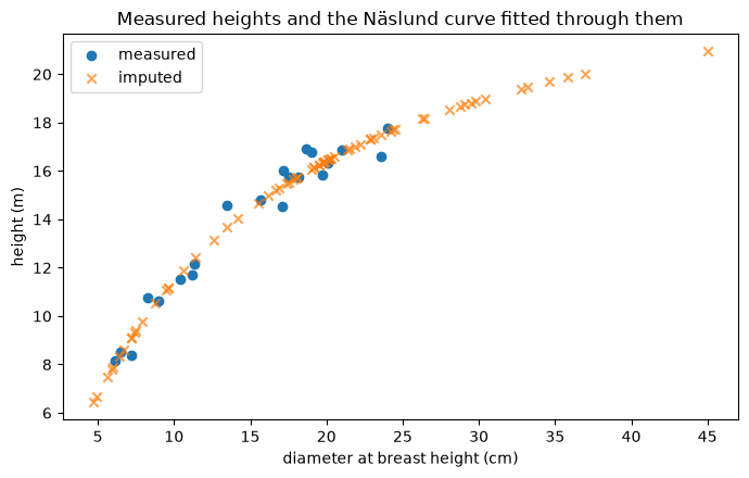
The imputed points lie exactly on the fitted curve, which is what an interpolated value is – it carries no residual scatter. The measured points scatter around it. Anything that treats the two alike will understate the variance it is working with.
3. Competition indices#
competition_indices takes a plot (or a stand, or a plain list of trees), the indices you want, and a rule for choosing competitors. Here are three indices with contrasting behaviour:
``Heg`` (Hegyi 1974) – distance-dependent size ratio; higher means more competition.
``BAL`` (Wykoff et al. 1982) – basal area of larger trees, distance independent.
``drg`` (Hamilton 1986) – the subject’s diameter over the plot’s quadratic mean diameter. Note this one runs the other way: a high value means the subject dominates.
[6]:
plot = stand.plots[0]
results = competition_indices(
    plot,
    indices=["Heg", "BAL", "drg"],
    selector=FixedRadius(8.0, min_size_ratio=0.3),
)

table = pd.DataFrame(
    {
        "uid": [r.tree.uid for r in results],
        "dbh_cm": [float(r.tree.diameter_cm) for r in results],
        "n_comp": [r.n_competitors for r in results],
        **{name: [r.indices[name] for r in results] for name in ("Heg", "BAL", "drg")},
    }
).sort_values("dbh_cm")

print(table.head(5).round(3).to_string(index=False))
print("   ...")
print(table.tail(5).round(3).to_string(index=False))
  uid  dbh_cm  n_comp    Heg    BAL   drg
p1t37     4.7      19 24.554 39.106 0.252
p1t31     4.9      29 31.089 39.046 0.263
p1t02     5.6      13 23.026 38.968 0.300
p1t20     5.9      19 26.137 38.881 0.316
p1t28     6.1      24 20.130 38.788 0.327
   ...
  uid  dbh_cm  n_comp   Heg   BAL   drg
p1t29    24.4      24 5.038 9.669 1.308
p1t25    26.3      12 3.517 7.939 1.410
p1t11    26.4      21 3.837 6.197 1.415
p1t44    34.6      10 3.183 3.204 1.854
p1t34    35.8      11 1.814 0.000 1.919
Small trees carry high Heg and BAL and low drg; large trees the reverse. That is the sanity check you want – a suppressed stem is under more competition than a dominant one.
n_comp counts the competitors the selector kept, and it drives Heg only. BAL and drg are plot descriptors: they are computed over every other tree on the plot whatever the selector does, which is what makes BAL comparable between runs that used different selection rules.
In the correlation below, drg sits at exactly 1.000 against diameter. That is not a finding: drg is the subject’s diameter divided by a plot-level constant, so within one plot it is diameter on a different scale. It earns its place as a predictor across plots of differing size, not within one.
[7]:
print(table[["dbh_cm", "Heg", "BAL", "drg"]].corr().round(3).to_string())
        dbh_cm    Heg    BAL    drg
dbh_cm   1.000 -0.870 -0.924  1.000
Heg     -0.870  1.000  0.692 -0.870
BAL     -0.924  0.692  1.000 -0.924
drg      1.000 -0.870 -0.924  1.000
4. The selection rule is part of the index#
An index value is only interpretable next to the rule that chose its competitors. The same Heg formula on the same plot gives materially different numbers under different rules, so the rule has to be reported alongside the index.
[8]:
selectors = {
    "FixedRadius(8 m)": FixedRadius(8.0),
    "MeanHeightRadius(0.4)": MeanHeightRadius(0.4),
    "MeanHeightRadius(0.25)": MeanHeightRadius(0.25),
    "LeeGadowRadius(k=2)": LeeGadowRadius(2.0),
    "LeeGadowRadius(k=3)": LeeGadowRadius(3.0),
    "BitterlichBAF(2)": BitterlichBAF(2.0),
    "NearestNeighbours(4)": NearestNeighbours(4),
    "SearchCone(80 deg)": SearchCone(80.0),
}

rows = []
for label, selector in selectors.items():
    res = competition_indices(plot, indices=["Heg"], selector=selector)
    src = selector_source(selector)
    rows.append(
        {
            "selector": label,
            "mean_competitors": sum(r.n_competitors for r in res) / len(res),
            "mean_Heg": sum(r.indices["Heg"] for r in res) / len(res),
            "citation": f"{src.author.split(',')[0]} {src.year}" if src else "(plain geometry)",
        }
    )

print(pd.DataFrame(rows).round(3).to_string(index=False))
              selector  mean_competitors  mean_Heg         citation
      FixedRadius(8 m)            18.533    10.012 (plain geometry)
 MeanHeightRadius(0.4)            10.578     6.891        Sims 2009
MeanHeightRadius(0.25)             4.444     4.191        Sims 2009
   LeeGadowRadius(k=2)             9.067     6.283         Lee 1997
   LeeGadowRadius(k=3)            18.133     9.868         Lee 1997
      BitterlichBAF(2)            13.000     6.066  Bitterlich 1952
  NearestNeighbours(4)             4.000     3.209 (plain geometry)
    SearchCone(80 deg)            31.289     8.765    Pretzsch 2009
Note how far apart these are. Every number in these rules is a parameter with a literature default, not a constant: MeanHeightRadius(0.4) uses the fraction Sims et al. (2009) tested, and dropping it to 0.25 shrinks the zone and the index with it.
SearchCone looks indiscriminate here, and at this scale it is: an 80 degree cone reaches h / tan(50 deg) horizontally, so a 20 m neighbour competes out to almost 17 m – further than this 10 m plot is wide. The cone discriminates on larger neighbourhoods, or at a narrower angle.
SearchCone and BitterlichBAF are the two rules whose reach depends on the neighbour’s size rather than the subject’s – the cone on its height, the angle gauge on its diameter. That is what a variable-radius rule means: under BitterlichBAF(2) a 60 cm neighbour competes out to 21 m while a 10 cm one stops at 3.5 m. Neither defines a single competition zone, so neither reports a zone_radius_m, and neither is edge-corrected – see section 5.
The two screens#
The comparison this set is drawn from applies two screens together for its influence-zone approaches: a neighbour must be at least 30% of the subject’s diameter, and must not stand in the shadow of a nearer competitor within 30 degrees. Reproducing those approaches needs both.
[9]:
screens = {
    "no screens": FixedRadius(8.0),
    "size only (0.3)": FixedRadius(8.0, min_size_ratio=0.3),
    "shadow only (30 deg)": FixedRadius(8.0, elimination_angle_deg=30.0),
    "both": FixedRadius(8.0, min_size_ratio=0.3, elimination_angle_deg=30.0),
}
for label, selector in screens.items():
    res = competition_indices(plot, indices=["Heg"], selector=selector)
    mean_n = sum(r.n_competitors for r in res) / len(res)
    mean_h = sum(r.indices["Heg"] for r in res) / len(res)
    print(f"{label:24s} mean competitors {mean_n:5.2f}   mean Heg {mean_h:6.3f}")
no screens               mean competitors 18.53   mean Heg 10.012
size only (0.3)          mean competitors 16.98   mean Heg  9.856
shadow only (30 deg)     mean competitors  9.11   mean Heg  6.849
both                     mean competitors  8.76   mean Heg  6.888
5. Edge correction#
A tree near the plot boundary has part of its competition zone outside the plot, so its distance-dependent indices come out too low. Each result reports observed_zone_fraction, the share of the zone that was actually inside, and by default the spatial indices are divided by it.
[10]:
raw = competition_indices(
    plot, indices=["Heg"], selector=FixedRadius(8.0), edge_correction=None
)
corrected = competition_indices(plot, indices=["Heg"], selector=FixedRadius(8.0))

edge = pd.DataFrame(
    {
        "uid": [r.tree.uid for r in raw],
        "dist_from_centre_m": [
            round(((r.tree.position.X - plot.position.X) ** 2
                   + (r.tree.position.Y - plot.position.Y) ** 2) ** 0.5, 2)
            for r in raw
        ],
        "observed_fraction": [round(r.observed_zone_fraction, 3) for r in raw],
        "Heg_raw": [round(r.indices["Heg"], 3) for r in raw],
        "Heg_corrected": [round(r2.indices["Heg"], 3) for r2 in corrected],
    }
).sort_values("dist_from_centre_m")

print("Trees nearest the plot centre (zone fully observed):")
print(edge.head(3).to_string(index=False))
print("\nTrees nearest the boundary (zone partly outside):")
print(edge.tail(3).to_string(index=False))
Trees nearest the plot centre (zone fully observed):
  uid  dist_from_centre_m  observed_fraction  Heg_raw  Heg_corrected
p1t05                0.73              1.000    5.119          5.119
p1t28                1.43              1.000   20.130         20.130
p1t14                2.41              0.986    5.349          5.427

Trees nearest the boundary (zone partly outside):
  uid  dist_from_centre_m  observed_fraction  Heg_raw  Heg_corrected
p1t02                9.43              0.455   10.486         23.026
p1t18                9.45              0.454    8.708         19.171
p1t01                9.96              0.417    4.036          9.682
Only the boundary trees change; a tree whose whole zone is inside the plot has observed_fraction == 1.0 and is left alone.
Three things are deliberately not corrected:
Non-spatial indices.
BALand its relatives are plot-level sums and do not depend on where in the plot the subject sits. They also ignore the selector entirely:BALis the basal area per hectare in trees larger than the subject over the whole plot, so it does not shrink when the search radius does.``SBAr`` and ``Almdg``. A ratio and a weight-normalised mean of areas do not scale with the observed share – halving the competitor set leaves both unchanged – so dividing them would invent competition.
INDEX_REGISTRY[name].additivesays which indices the correction applies to.Selections with no zone fixed in advance (
SearchCone,NearestNeighbours,BitterlichBAF). Their reach is an outcome of the data, and a neighbourhood truncated by the boundary reaches less far – so using it to size the correction would under-correct by exactly the amount at issue.
6. Where the numbers come from#
Every index carries the citation of the paper that proposed it – not the review they were collected from. That means a result can always answer “according to whom?”.
[11]:
catalogue = pd.DataFrame(
    [
        {
            "index": name,
            "spatial": entry.spatial,
            "author": index_source(name).author,
            "year": index_source(name).year,
        }
        for name, entry in INDEX_REGISTRY.items()
    ]
).sort_values(["spatial", "year"])
print(catalogue.to_string(index=False))
 index  spatial                                       author  year
 BA-gj    False                Steneker, G.A. & Jarvis, J.M.  1963
   BAL    False  Wykoff, W.R., Crookston, N.L. & Stage, A.R.  1982
   Sdr    False                                Lorimer, C.G.  1983
   drg    False                               Hamilton, D.A.  1986
   BAr    False                     Corona, P. & Ferrara, A.  1989
  BALr    False                                Vanclay, J.K.  1991
BALMOD    False                 Schröder, J. & von Gadow, K.  1999
    Sl     True                               Staebler, G.R.  1951
   SOr     True                                Gerrard, D.J.  1969
  SOdr     True                                  Bella, I.E.  1971
   Heg     True                                    Hegyi, F.  1974
 SAng1     True                                    Lin, J.Y.  1974
 Almdg     True                                Alemdag, I.S.  1978
 Sdrl1     True                                Lorimer, C.G.  1983
 Sdrl2     True                      Martin, G.L. & Ek, A.R.  1984
  SBAr     True Daniels, R.F., Burkhart, H.E. & Clason, T.R.  1986
 SAng2     True               Rouvinen, S. & Kuuluvainen, T.  1997
SdrAng     True               Rouvinen, S. & Kuuluvainen, T.  1997
Summary#
Stand.impute("height_m")fits Näslund’s curve to the stand’s own measured pairs and fills the gaps, keeping measured and modelled values distinct and recording which model produced each modelled one.competition_indices(...)computes any of the eighteen indices; passindices=to choose andselector=to say how competitors are found.The selection rule is part of the result. Report it alongside the index, and treat its parameters as parameters – the defaults are one study’s choices.
Distance-dependent indices are biased low at the plot edge;
observed_zone_fractionreports the exposure and the default corrects for it.
Next steps#
The influence-zone indices (
Sl,SOr,SOdr) additionally need a crown radius. Supply one withstand.impute("crown_radius_m", <callable>)or thecrown_radius=argument; a caller-supplied value is recorded as uncited.SearchCone(apex="crown_base")needscrown_base_height_m, which can be imputed the same way.